Play Time

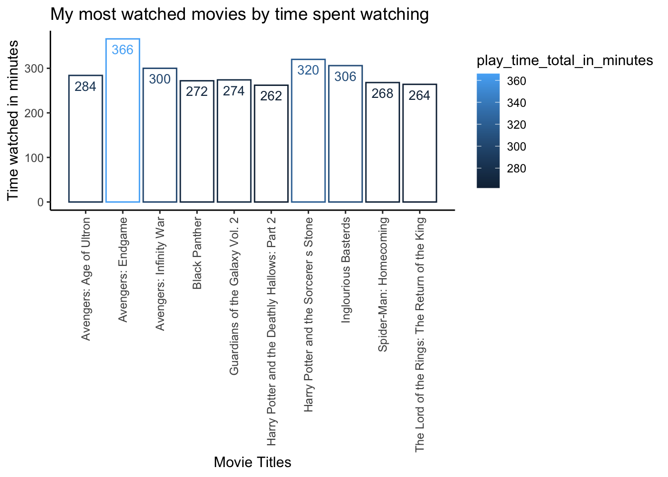
So I want to see with wich movies I have wasted the most amount of time.

To analyse all the movies throughout all the libraries, we first load the existing .csv files with the data from Plex. We then combine them into one giant data frame.

all_movie_libraries <- list.files(path = "data", pattern = "*.csv", full.names = TRUE) %>%
                              lapply(read.csv) %>%
                              lapply(\(x) mutate(x, across(Audience.Rating, as.double))) %>%
                              bind_rows()

We then change the Duration from the format HH:MM:SS to an amount in minutes. Also we discard a lot of columns we don’t need anymore.

all_movie_libraries <- all_movie_libraries %>%
                                separate(Duration, c('play_time_hours', 'play_time_minutes', 'play_time_seconds'), ':') %>%
                                mutate(play_time_hours = as.numeric(play_time_hours), play_time_minutes = as.numeric(play_time_minutes), play_time_seconds = as.numeric(play_time_seconds)) %>%
                                mutate(play_time_single_in_minutes = ceiling(play_time_hours*60 + play_time_minutes + play_time_seconds/60)) %>%
                                select(title = Title,view_count = View.Count, play_time_single_in_minutes)
                                
head(all_movie_libraries)

##                                    title view_count play_time_single_in_minutes
## 1                            Animal Farm        N/A                          73
## 2           Batman & Mr. Freeze: SubZero        N/A                          68
## 3                           Batman Ninja        N/A                          86
## 4 Batman vs Teenage Mutant Ninja Turtles        N/A                          88
## 5                 The Batman vs. Dracula          1                          85
## 6                    Batman vs. Two-Face          1                          73

Now let’s filter out all movies that haven’t been watched before.

all_movie_libraries = all_movie_libraries %>%
                          filter(view_count != 'N/A')

With this we reduced the rows in our data frame from 869 to 287.

After that we multiply the amount of minutes with the amount of times the movie has been played. This gives us the total amount of time played.

all_movie_libraries <- all_movie_libraries %>%
                        mutate(view_count = as.numeric(view_count)) %>%
                        mutate(play_time_total_in_minutes = play_time_single_in_minutes * view_count) %>%
                        select(title, play_time_total_in_minutes)

head(all_movie_libraries)

##                          title play_time_total_in_minutes
## 1       The Batman vs. Dracula                         85
## 2          Batman vs. Two-Face                         73
## 3    Batman: Assault on Arkham                        154
## 4            Batman: Bad Blood                        148
## 5                 Batman: Hush                         83
## 6 Batman: Mask of the Phantasm                         77

And now sort the data frame in a descending order, pick the top 10 rows and make a bar plot.

all_movie_libraries <- all_movie_libraries %>%
                        arrange(desc(play_time_total_in_minutes)) %>%
                        head(10)

all_movie_libraries %>% 
  ggplot(aes(x=title, y=play_time_total_in_minutes, color=play_time_total_in_minutes)) +
    geom_bar(stat="identity", fill="white") +
    scale_x_discrete(guide = guide_axis(angle = 90)) +
    geom_text(aes(label=play_time_total_in_minutes), position = position_dodge(1.9), size=3.5, vjust=1.6) +
    labs(title = 'My most watched movies by time spent watching', y = 'Time watched in minutes', x = 'Movie Titles') +
    theme_classic()