Audience/Critic Rating

Let’s see if the movies on my Plex server are even any good.

To analyse all the movies throughout all the libraries, we first load the existing .csv files with the data from Plex. We then combine them into one giant data frame.

all_movie_libraries <- list.files(path = "data", pattern = "*.csv", full.names = TRUE) %>%
                              lapply(read.csv) %>%
                              lapply(\(x) mutate(x, across(Audience.Rating, as.double))) %>%
                              bind_rows()

We will now filter out all the unused columns and also all the movies which haven’t got an audience and/or critic rating.

all_movie_libraries <- all_movie_libraries %>%
                        select(title = Title, critic_rating = Rating, audience_rating = Audience.Rating) %>%
                        filter(critic_rating != 'N/A', audience_rating != 'N/A') %>%
                        mutate(critic_rating = as.numeric(critic_rating), audience_rating = as.numeric(audience_rating))
head(all_movie_libraries)

##                                    title critic_rating audience_rating
## 1                            Animal Farm           6.9             6.6
## 2           Batman & Mr. Freeze: SubZero           9.2             6.7
## 3                           Batman Ninja           8.2             6.1
## 4 Batman vs Teenage Mutant Ninja Turtles          10.0             8.6
## 5                    Batman vs. Two-Face          10.0             6.1
## 6              Batman: Assault on Arkham           7.5             8.5

This brings us down from 869 to 810 movies. This is now pretty nice to look at but won’t work with ggplot2. For that the data has to be transformed from “wide” to “long”. Like that:

wide_data <- all_movie_libraries %>%
                gather('critic_rating','audience_rating', key='rating_type', value='rating')

This means we now have two rows for each movie:

print(wide_data %>% filter(title == 'Animal Farm'))

##         title     rating_type rating
## 1 Animal Farm   critic_rating    6.9
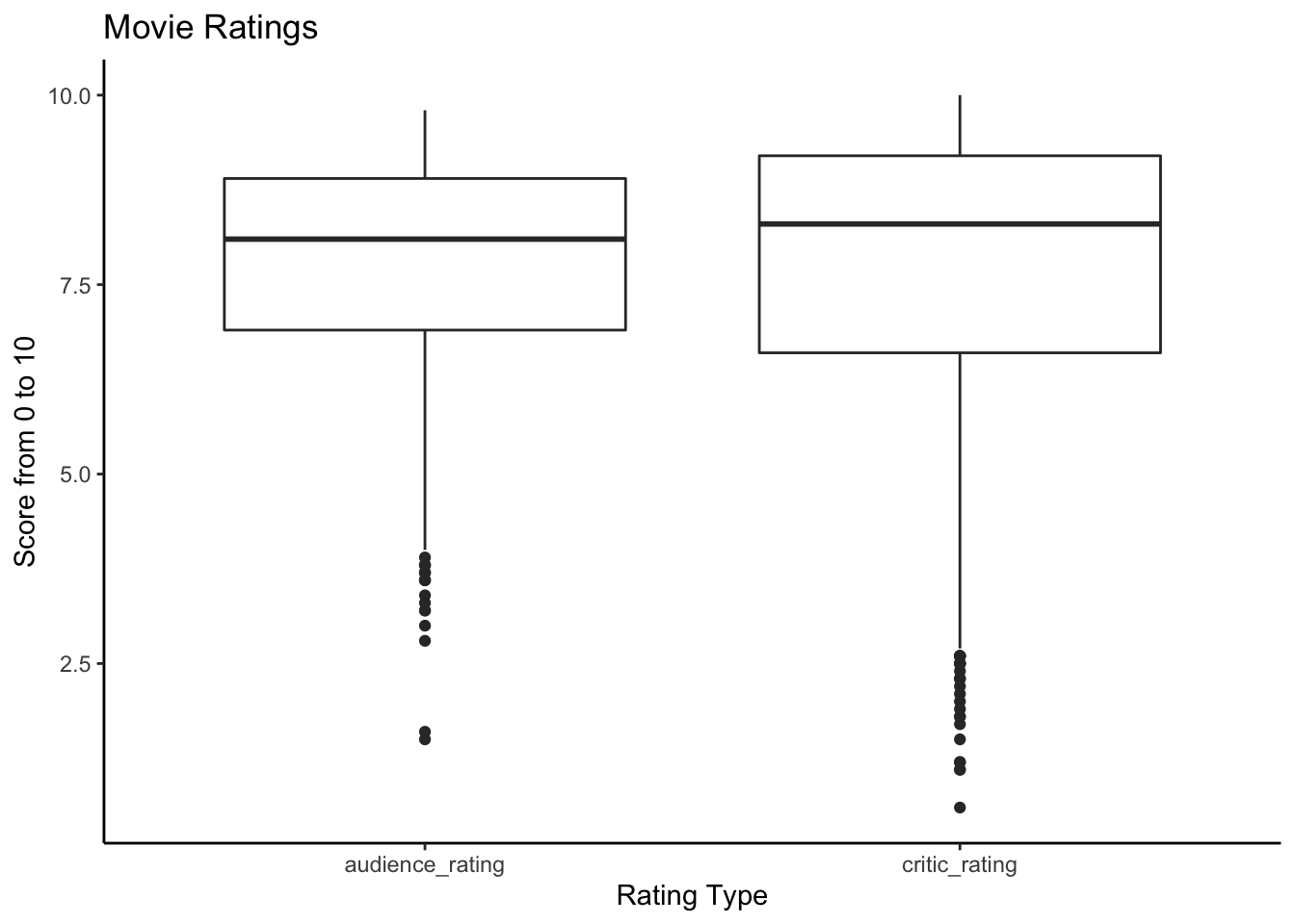
## 2 Animal Farm audience_rating    6.6

With this ggplot2 can now generate a nice box plot.

wide_data %>%
  ggplot(aes(y = rating, x = rating_type)) +
  geom_boxplot() +
  labs(title = 'Movie Ratings', y = 'Score from 0 to 10', x = 'Rating Type') +
  theme_classic()

We can see a couple things here:
1. That I have a pretty good taste in movies, with the critic rating median being 8.3 and the audience median being 8.1.
2. That the critic and audience are generally in agreement.
3. That there are many out liners on the “not-so-good-a-score” side.

I want to take a closer look at the last point some more code that we can use for an informative table:

#Using two functions because I could not get the column name as an argument to work
get_movie_amount_critic <- function(score){
  amount <- nrow(all_movie_libraries %>%
                  filter(critic_rating <= score))
  return(paste0(amount, ' (', get_percent(amount), '%)'))
} 


get_movie_amount_audience <- function(score){
  amount <- nrow(all_movie_libraries %>%
                  filter(audience_rating <= score))
  return(paste0(amount, ' (', get_percent(amount), '%)'))
} 

get_percent <- function(value){
  return(round((value * 100)/nrow(all_movie_libraries), digits=2))
}

lowest_score_row_critic <- all_movie_libraries[which.min(all_movie_libraries$critic_rating),]
lowest_score_row_audience <- all_movie_libraries[which.min(all_movie_libraries$audience_rating),]

	Critic Rating	Audience Rating
Amount of movies with rating < 5.0	98 (12.1%)	67 (8.27%)
Amount of movies with rating < 2.5	20 (2.47%)	2 (0.25%)
Amount of movies with rating < 1.0	1 (0.12%)	0 (0%)
Lowest scoring movie	RoboCop 3 with a score of 0.6	RoboCop 3 with a score of 1.5